Continued from Artificial Intelligence for Children Part 3

So, we now know something about AI and Machine Learning and we have also got an idea of how it works.

In our discussion today, let us do a simple Machine Learning problem ourselves.

To begin with, you will need an environment (to write the code, access the libraries that have been designed by researchers, compile the code for the computer to understand it) to write the ML program. While there are ways to install various libraries in your computer, we will take a simpler route. There are certain platforms such as www.kaggle.com that offer web-based, ready-to-code environments for AI enthusiasts.

Step 1: Register/ Sign in to Kaggle (a great platform to work on AI problems and to participate in competitions)

Next we need to define the problem we want to solve and we will need data. This is an important point – for machine learning problems, we will need data to ‘train’ the machines.

Step 2: Go to https://www.kaggle.com/uciml/iris#

The problem that we are trying to solve using Machine Learning is as follows –

Assume that you own a garden that has 3 different types of flowers. While you can identify those flowers quickly, machines cannot. They need to learn before they can identify. So, we will have to train our machine to understand the characteristics of the 3 flowers. Once the machine has learnt the different characteristics, when it sees a new flower, it will be able to tell which type the flower belongs to.

So, you collect data to teach the machine. For this, you have taken 50 flowers of each type and have put down 4 properties of each flower in a table i.e. Petal Length, Petal Width, Sepal Length and Sepal Width. Of course, you have also mentioned the type (or species) for each of the flower. The 3 species in your garden are – Setosa, Versicolor and Virginica.

Luckily, this data is available here on Kaggle and you don’t need to go to the garden to collect it.

Step 3: Create a ‘New Notebook’ and select ‘Python’ language and ‘Notebook options’

The notebook is the place where we will write our code. So, with the above steps, now you have –

• An environment to run Python code i.e. a Jupyter notebook
  1. here you can code in Python
  2. you have access to all the Machine Learning libraries that you will need for this assignment
  3. you can compile and run the code i.e. make the computer understand what needs to be done
• Data on 150 flowers (50 flowers each of 3 species). We will use a part of this data to ‘train’ our machine and rest of the data to ‘test’ the machine if it has learnt the lesson well 😊

Step 4: Let’s write the code now. Note that we are keeping a very simple, minimal code at this stage just to demonstrate how the machines learn and are able to take decisions. There can be lot more steps that will improve the results of our machine but, for now, we will keep it as simple as possible.

The notebook that is now in front of you comprises of ‘cells’ (as shown in the below image) where you can write your code. After writing your code, from within the cell, press ‘Shift + Enter’ which will run the code in the cell and give the results below the cell. You can move to the next cell below to writer further code and run it.

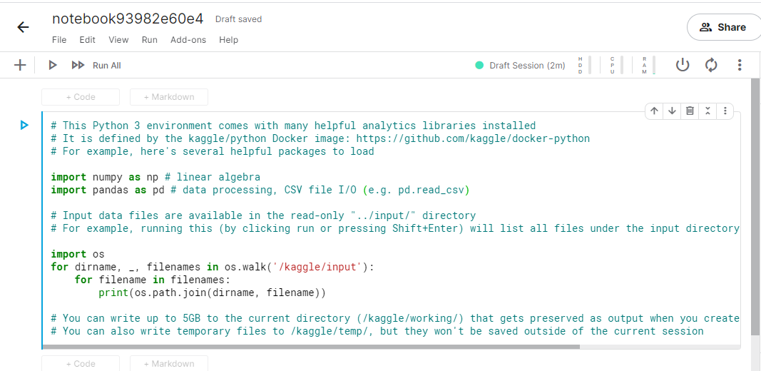
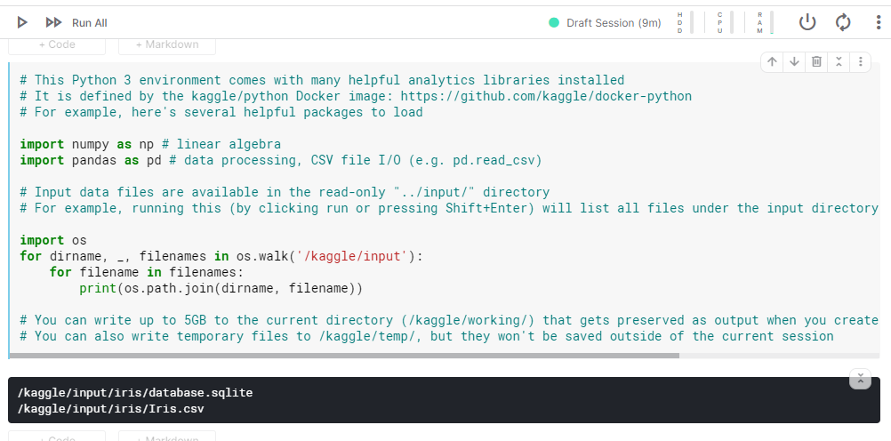
On running the code in the cell, we get the output. So, your Python code is running. All that has been done is that we have imported libraries called numpy and pandas (that consist of pre-written code that is useful for machine learning problems) and have asked for the data files that are available to us.

Note that we have a file called Iris.csv which is the data on 150 flowers that we will use for our problem.

In the next cell, let us write –

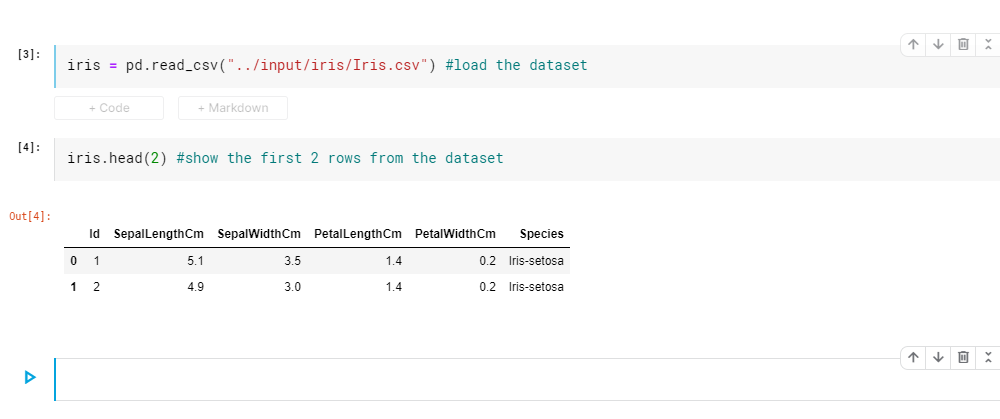
iris = pd.read_csv(“../input/iris/Iris.csv”) #load the dataset

iris.head(2) #show the first 2 rows from the dataset

Here we are reading the file that has the data on the 150 flowers and then looking at what data is available for the first 2 flowers.

Next we will drop the ID column from this data table as it is not representing the flower in any way. We can check the data on first 2 flowers again to see that the Id column has been dropped.

iris.drop(‘Id’,axis=1,inplace=True) #dropping the Id column as it is unnecessary

iris.head(2) #show the first 2 rows from the dataset

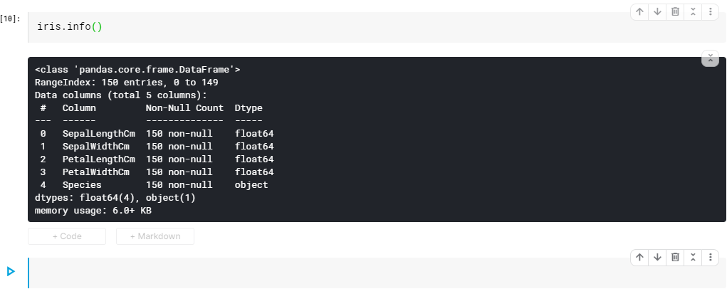
Note that in the data that we have on the flowers, as we had discussed earlier, there are 4 features that are being used to identify the flower type – Sepal Length, Sepal Width, Petal Length and Petal Width.  The species could be one of the three – Setosa, Versicolor and Virginica. The features are the ‘Predictor Variables’ and species in this case is the ‘Predicted Variable’.

Let us check this in the structure of the table as follows.

iris.info()

At this point of time, we have data on 150 flowers (50 flowers of each of the 3 types). Before we train our machine to start understanding the difference of the flower types, we split the entire data into a training set and a test set. We would train the machine on one part of the data and then test the machine on the other data to see how accurately can the machine identify the flowers during the test.

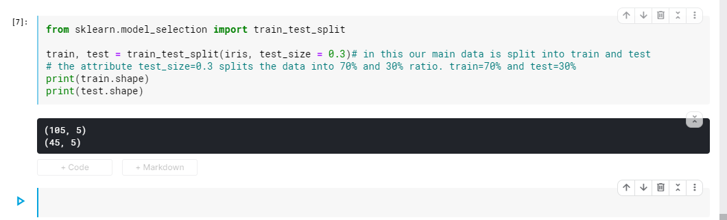
To split the data, we want that the training data and test data should be randomly selected but both should have reasonable representation of all the 3 types of flowers. For this we would use a utility that is pre-coded in a library publicly available to us. The library is call sklearn and the utility is called train_test_split. We will split the data such that 70% of it is available for training and we test the machine on remaining 30%.

Let’s also check how the new datasets, train and test, look like i.e. how many flowers are available in the two datasets after the split. We see that 105 flowers’ data is in train and 45 in test.

from sklearn.model_selection import train_test_split

train, test = train_test_split(iris, test_size = 0.3)# in this our main data is split into train and test

# the attribute test_size=0.3 splits the data into 70% and 30% ratio. train=70% and test=30%

print(train.shape)

print(test.shape)

Now we need to tell our Machine Learning models, which columns in the data are the Predictor Variables and which is the Predicted Variable. We need to provide this information for both training data and for the testing data.

train_X = train[[‘SepalLengthCm’,’SepalWidthCm’,’PetalLengthCm’,’PetalWidthCm’]]# taking the training data features

train_y=train.Species# output of our training data

test_X= test[[‘SepalLengthCm’,’SepalWidthCm’,’PetalLengthCm’,’PetalWidthCm’]] # taking test data features

test_y =test.Species   #output value of test data

Now we are ready to use some algorithms (machine learning programs that researchers have written that can look at patterns in the data and generate the best fit function between predictor and predicted variables) to train the machine and see how good the machine is learning. We will use 2 different algorithms here (Logistic Regression and Support Vector Machine or SVM) thought there are many more that could be tried if these do not give good results.

The steps that we are following here are –

• Import the algorithms that we need to use in our program
• Use Logistic Regression and SVM algorithms to train the model on train data
• Run the models on Test data and get the prediction from the models
• Print the accuracy that the machine is able to get on the Test data – accuracy being defined as how many of the flower species are accurately identified by the machine

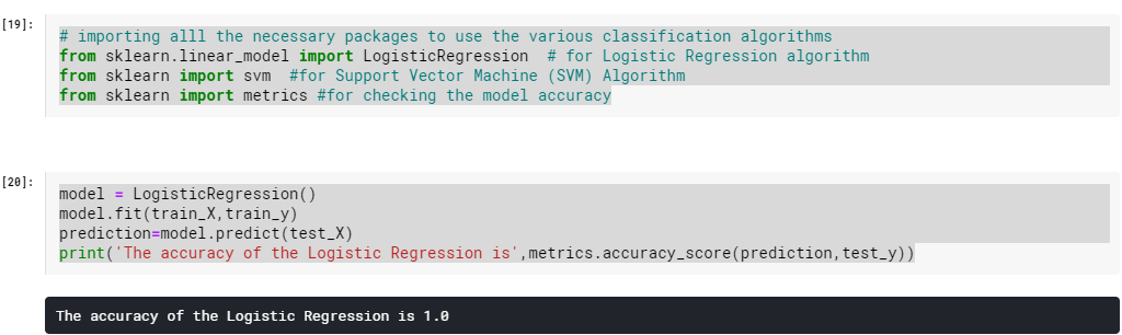
# importing alll the necessary packages to use the various classification algorithms

from sklearn.linear_model import LogisticRegression  # for Logistic Regression algorithm

from sklearn import svm  #for Support Vector Machine (SVM) Algorithm

from sklearn import metrics #for checking the model accuracy

model = LogisticRegression()

model.fit(train_X,train_y)

prediction=model.predict(test_X)

print(‘The accuracy of the Logistic Regression is’,metrics.accuracy_score(prediction,test_y))

model = svm.SVC() #select the algorithm

model.fit(train_X,train_y) # we train the algorithm with the training data and the training output

prediction=model.predict(test_X) #now we pass the testing data to the trained algorithm

print(‘The accuracy of the SVM is:’,metrics.accuracy_score(prediction,test_y))#now we check the accuracy of the algorithm.

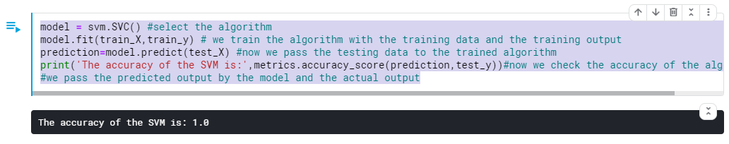
What we see is that in both the algorithms above, the accuracy is 1.0 or 100%. So, the models are good enough that they can predict the flowers with almost no error. If now we use one of the models and give the features (Sepal and Petal length and width) of a new flower, the model will be able to identify the specie of the flower with good accuracy.

Congratulations -you have made a real Machine Learning program and now your machine can make intelligent decision without any manual intervention!

Before we conclude, I would like to share that there are various types of problems that can be managed with Machine Learning and Deep Learning techniques today. There are a lot of ways that the accuracy of predictions can be improved (we saw a 100% accuracy above but that is normally not the case) and we could see some of them in our coming sessions.

However, the good thing is that the key steps of all the programs (even if you are building a self-driving car) will remain the same as what you have already done.

So, happy learning dear, budding Data Scientist!